Demystifying diffusion models

If you haven’t been living under a rock you might have seen the phenomenal capabilities of the recent DALL.E model released by OpenAI. This model can generate new images based on a simple text prompt, What a time to be alive ! DALL.E 2 can make high-quality novel images from just a text input and just look how creative can it get !! Many other similar models have been released in the recent past including Midjourney, Stable Diffusion etc.

You must be wondering how exactly does DALL.E or Midjourney do it? The answer is “Diffusion Models” !!!. Let’s take a deep-dive into, how exactly do these diffusion models work.

In this blog, we will study the basic principles that drive the diffusion models. There are a lot of new architectures in the diffusion models family, which can be a little overwhelming. We will focus on the most initial and prominent of them, Denoising Diffusion Probabilistic Models i.e. DDPMs by Sohl-Dickstein et al. and then proposed by Ho et al.

The underlying idea: the diffusion process#

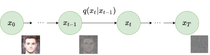
The basic idea behind Diffusion models is simple they take an input image $x_0$ from a data distribution and gradually add gaussian noise to it over $T$ timesteps. This is inspired from the Diffusion Process in thermodynamics, which is defined as the “spreading” of particles from regions of higher concentrations to lower concentration. This process of perturbing the input image with gaussian noise over $T$ timesteps is called the forward process.

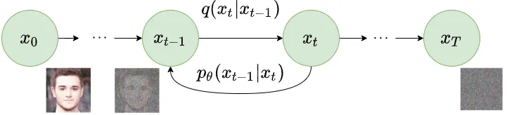
After the forward process a neural network is trained to recover the original image by reversing the noising process. This is called the reverse process or the sampling of the generative model. Using the learned information we can generate novel samples from the trained diffusion model.

Let us look into the underlying maths to make things crystal clear!

Forward process#

Diffusion models are viewed similar to latent variable models similar to Variational Autoencoders (VAEs) which have a continuous hidden latent space.

Diffusion models are modelled using a Markov chain having $T$ steps. In Markov chains, each step only depends on the previous step. These Markov chain form the underlying assumption in the Diffusion models.

We take a datapoint $x_0$ from a data distribution $q(x)$, we can define a forward diffusion process by adding noise. At each step $t < T$ we add gaussian noise with some variance $\beta_t$ to the datapoint $x_{t-1}$, this produces a new datapoint $x_t$ with a distribution $q(x_t | x_{t-1})$. This variance follows some fixed schedule (cosine or linear or any other). In the original DDPM paper they choose $\beta_t$ to follow a linear schedule ranging from 0.0001 to 0.02.¹1Nichol & Dhariwal later showed that a cosine schedule works better. With the linear one, the last steps are already close to pure noise, so they teach the model very little. This forward diffusion process can be formulated by:

$$\boxed{q(x_t|x_{t-1}) := \mathcal{N}(x_t; \sqrt{1-\beta_t}\,x_{t-1}, \beta_t I)}$$

Note that $q(x_t | x_{t-1})$ is still a normal distribution. Thus we can go from $x_0$ to $x_T$ in a tractable manner, this is given by the equation:

$$\boxed{q(x_{1:T}|x_0) = \prod_{t=1}^T q(x_t|x_{t-1})}$$

This is also known as the posterior probability. Here $q(x_{1:T})$ means we apply the same process from time step 1 to $T$. But this means that in order to get $x_t$ at a certain time step t=200 we will have to apply the forward diffusion process 200 times to the input $x_0$. Well this can be lets say… computationally taxing! But to overcome this problem we have a cool trick up our sleeve!!

The reparameterization trick#

Instead of applying the forward process many times repeatedly to get the desired datapoint $x_t$ at $t < T$, we can apply this simple reparameterization to get the desired output by simply precomputing the variances and certain parameters.

Let us define $\alpha_t = 1-\beta_t$ and $\bar{\alpha}_t = \prod_{i=1}^{t} \alpha_i$ where $\epsilon \sim \mathcal{N}(0, I)$. Using this we can sample $x_t$ at any $t$, using this trick:

jump straight to any t ↓ $$\boxed{x_t = \sqrt{\bar{\alpha}_t}\,x_0 + \sqrt{1-\bar{\alpha}_t}\,\epsilon}$$

Why does this work? (the two-line derivation)

Write one step as $x_t = \sqrt{\alpha_t}\,x_{t-1} + \sqrt{1-\alpha_t}\,\epsilon_{t-1}$ and plug in the same expression for $x_{t-1}$:

$$x_t = \sqrt{\alpha_t \alpha_{t-1}}\,x_{t-2} + \sqrt{\alpha_t(1-\alpha_{t-1})}\,\epsilon_{t-2} + \sqrt{1-\alpha_t}\,\epsilon_{t-1}$$

The two noise terms are independent Gaussians, so their sum is one Gaussian with variance $\alpha_t(1-\alpha_{t-1}) + (1-\alpha_t) = 1 - \alpha_t\alpha_{t-1}$. Keep unrolling down to $x_0$ and the product of all the $\alpha$s is $\bar{\alpha}_t$.

Thus to put it more mathematically we can produce a sample $x_t$ using this distribution:

$$\boxed{q(x_t|x_0) = \mathcal{N}(x_t; \sqrt{\bar{\alpha}_t}\,x_0, (1-\bar{\alpha}_t)I)}$$

As discussed earlier we can precompute $\beta_t$, $\alpha_t$, and $\bar{\alpha}_t$ at all timesteps. Thus we can sample $x_t$ arbitrarily at any timestep, we will use this “nice” property later in defining the training objective for our model. Try it below. Every frame is one evaluation of the equation above, not 200 steps of noise.

Interactivedrag t!

x_t

t

0

PlayNew noise

β_t0

ᾱ_t1

signal √ᾱ_t1

noise √(1−ᾱ_t)0

Reverse diffusion#

When $T \to \infty$, we approach an isotropic gaussian distribution, i.e with a diagonal variance matrix. Now if we learn the reverse distribution $q(x_{t-1} | x_t)$ we can iteratively sample a novel datapoint with a starting prior distribution $x_T$ from $\mathcal{N}(0, I)$.

Let us see how can we model the reverse distribution.

Approximating reverse diffusion using a neural network#

The reverse distribution $q(x_{t-1} | x_t)$ is practically intractable as calculating it involves the whole data distribution. Instead we can approximate this by a parameterized model $p_\theta$, this can be a neural network. For a small enough $\beta_t$ we can choose $p_\theta$ to be a gaussian and parameterize its mean and variance.

$$\boxed{p_\theta(x_{t-1}|x_t) := \mathcal{N}(x_{t-1}; \mu_\theta(x_t, t), \Sigma_\theta(x_t, t))}$$

If we apply the reverse formula and additionally condition on timestep t we can make the model to predict the mean $\mu_\theta$ and the variance $\Sigma_\theta$ at each timestep.

Training the diffusion model#

As mentioned before diffusion models are similar to variational autoencoders (VAEs), now looking at the formulation of $q$ and $p$ we can clearly see the similarities. So similar to VAEs we can train it by maximizing the ELBO (Evidence Lower Bound) or the negative log-likelihood of the training data. We can write the ELBO as follows:

$$\boxed{L_{VLB} = \mathbb{E}_q \Big[ \underbrace{L_T}_{\text{constant}} + \sum_{t>1} \underbrace{D_{KL}(q(x_{t-1}|x_t, x_0) \,\|\, p_\theta(x_{t-1}|x_t))}_{L_{t-1}} - \underbrace{\log p_\theta(x_0|x_1)}_{L_0} \Big]}$$

Breaking down and analysing the objective:

• The $L_T$ term can be ignored as it is constant, q has no learnable parameters and $x_T$ is gaussian noise.
• The $L_0$ term can be modelled using a different decoder as a reconstruction term similar to the term in the ELBO of the VAE. Ho et al. modelled this term using a separate decoder.
• The $L_t$ term formulates the desired difference between the noising steps $q$ and denoising steps $p$.

It is evident that the objective function boils down to maximizing the $L_t$ term in the ELBO.

Using Bayes rule we can derive:

$$\boxed{q(x_{t-1}|x_t, x_0) = q(x_t|x_{t-1}, x_0) \frac{q(x_{t-1}|x_0)}{q(x_t|x_0)}}$$

The mean $\tilde{\mu}_t(x_t, x_0)$ can be written as:

$$\boxed{\tilde{\mu}_t(x_t, x_0) = \frac{\sqrt{\bar{\alpha}_{t-1}}\beta_t}{1-\bar{\alpha}_t}x_0 + \frac{\sqrt{\alpha_t}(1-\bar{\alpha}_{t-1})}{1-\bar{\alpha}_t}x_t}$$

Further we can make the $\mu$ in the above equation dependent on only $x_t$ by using the “nice” property we defined above:

$$\boxed{\tilde{\mu}_t = \frac{1}{\sqrt{\alpha_t}} \left( x_t - \frac{\beta_t}{\sqrt{1-\bar{\alpha}_t}}\epsilon_t \right)}$$

We have to make our network predict this $\mu_t$ via a parameterization of $\mu$ on $\theta$. Now the objective function in ELBO, $L_t$ can be further simplified as:

$$\boxed{L_t = \mathbb{E}_{x_0, \epsilon} \left[ \frac{\beta_t^2}{2\sigma_t^2 \alpha_t(1-\bar{\alpha}_t)} \|\epsilon - \epsilon_\theta(x_t, t)\|^2 \right]}$$

This loss function shows us that the model will learn to predict the noise $\epsilon$ at each timestep $t$, instead of predicting the mean at each timestep.

Ho et al. further simplified this objective by ignoring the weighing term in the above equation. They suggested this loss was enough to make the model learn its generative properties.

this one line is the whole trick ↙ $$\boxed{L_t^{\text{simple}} = \mathbb{E}_{t, x_0, \epsilon} \left[ \| \epsilon - \epsilon_\theta(\sqrt{\bar{\alpha}_t}x_0 + \sqrt{1-\bar{\alpha}_t}\epsilon, t) \|^2 \right]}$$

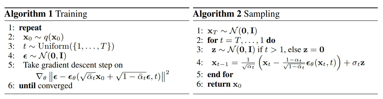
In code, one training step is just a few lines:

t = torch.randint(0, T, (batch_size,))  # a timestep per image
eps = torch.randn_like(x0)               # the noise we add
xt = a_bar[t].sqrt() * x0 + (1 - a_bar[t]).sqrt() * eps
loss = F.mse_loss(model(xt, t), eps)     # predict the noise

The detailed proofs to all the above equations are clearly explained in this great, must read article from Lilian Weng. Ho et al. also proposed to keep the posterior variance fixed instead of making the network predict that as well. This was further improved in Nichol et al.

The algorithms to train and sample the model as illustrated in Ho et al.:

Architecture#

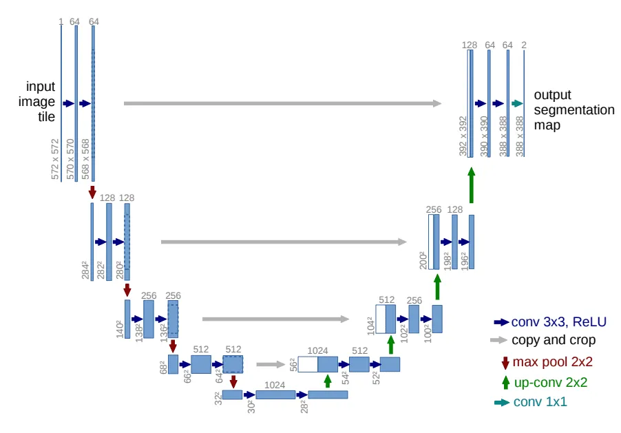
The neural network used to predict the noise and essentially model this diffusion process is an architecture very similar almost same to UNet, proposed by Ronneberger et al. in 2015 primarily for medical image segmentation. It is a symmetrical architecture with the inputs and outputs having the same dimensions. The networks also employ skip connections at each level. In the original implementation of DDPMs, UNet architecture with wide ResNet blocks, group normalization and self attention blocks is used.

Conclusion#

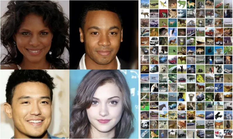
We successfully studied the working of the famous diffusion models in its original form, further more this architecture was iteratively improved conditioning it on additional information or using this architecture along with classifier-guidance, textual information. But the core principle of this method of modelling remains surprisingly same. These models have proven to generate great quality images with just a text prompt in any style, environment that we provide. Further improvements will definitely be seen in this promising method in different fields apart from just image generation!!

Further reading#

You can check out these excellent blogposts and papers to learn about diffusion and related research.

• “Denoising Diffusion Probabilistic Models” by Ho et al.
• “Improved Denoising Diffusion Probabilistic Models” by Nichol et al.
• “Denoising Diffusion Implicit Models” by Song et al.
• “How diffusion models work: the math from scratch”, a blogpost on AI Summer by Sergios Karagiannakos and Nikolas Adaloglou.
• “The Annotated Diffusion Model” on Hugging Face by Niels Rogge and Kashif Rasul.
• “Generative Modeling by Estimating Gradients of the Data Distribution”, a blogpost by Yang Song.

Footnotes#

1. Nichol & Dhariwal later showed that a cosine schedule works better. With the linear one, the last steps are already close to pure noise, so they teach the model very little. ↩